What if the points we want to sample do not live in ordinary 2D or 3D space? A dataset might describe each observation with dozens of measurements. Even a set of 3D coordinates can have a shape that straight-line distance describes poorly: points on opposite folds of a surface may be close through space but far apart along the surface. A representative subset needs a useful notion of neighborhood before it can decide where the gaps are.
My earlier void-and-cluster sampling project focused on large scattered datasets and time-dependent trajectories. It selects existing points, spreads them into a blue-noise-like pattern, and orders them for progressive loading. vc_sample explores how far the same selection procedure can go when the data is described by other coordinates or by a neighborhood graph.
The familiar spatial domain
The first image is the full 2D point set; the second retains 10% of its points. The subset fills the domain without the gaps and clumps that a small random selection can produce.
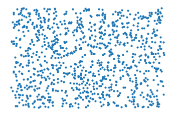
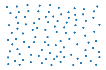
The method starts with a random subset. It then finds the largest void, an unselected point with little nearby sample coverage, and the tightest cluster, a selected point in an overcrowded neighborhood. Exchanging them improves the distribution. Once the initial subset has settled, the algorithm fills the remaining voids one at a time until it reaches the requested size. The order of those additions gives progressively larger subsets without starting over for each level of detail.
The important question is how to measure coverage. In the ordinary coordinate-space estimator, nearby points contribute through a Gaussian kernel. The implementation uses a spatial tree to find neighbors and can account for the density of all input points, so a naturally dense part of the dataset can still receive more samples. It also accepts importance weights when some regions should receive greater attention. The example notebook demonstrates 1D, 2D, and 3D sets, a noisy sine-shaped cloud, and nonuniform importance.
The sampling loop does not need coordinates
In the code, the void-and-cluster loop never inspects a point’s coordinates. It asks a density estimator for the current coverage score at every point and asks that estimator to update the scores when a sample is added or removed. The implementation calls these operations estimate, add, and sub.
This separation is the extension’s key idea. The selection rule can stay the same while the estimator defines what “nearby” means. For Euclidean point sets, it uses a kernel. For data whose structure is better described by local connections, it can use a weighted graph. The algorithm and two estimator implementations make that boundary visible in the code.
A surface inside a higher-dimensional space
The S-curve makes the distinction concrete. It is a two-dimensional surface folded through three-dimensional space. If a fixed-bandwidth kernel judges neighbors by straight-line 3D distance, a bandwidth large enough to connect points along the surface can also reach across folds. A bandwidth small enough to avoid those shortcuts may leave gaps. The higher-dimensional notebook shows this problem before trying a different estimator.
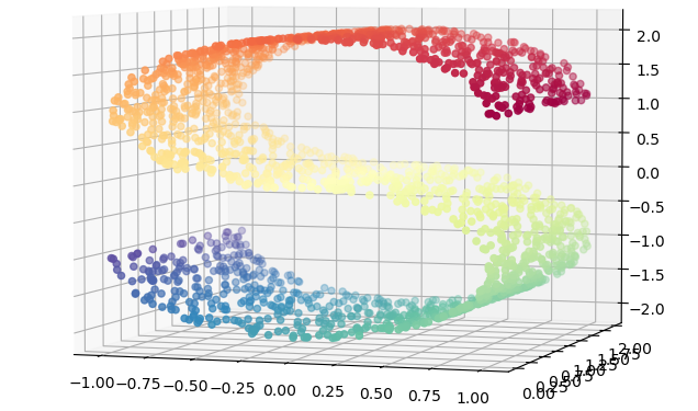
Figure 3. The full S-curve point set: a two-dimensional manifold embedded in 3D. Source: vc_sample.

The alternative estimator builds a weighted neighbor graph using UMAP’s fuzzy simplicial set construction. During sampling, adding a point changes the coverage scores of its graph neighbors rather than using a fixed-bandwidth kernel in 3D. The graph is still constructed from a chosen metric on the original coordinates; it is not a perfect reconstruction of the surface. But its local connections can represent this example’s folded structure more usefully for sampling.
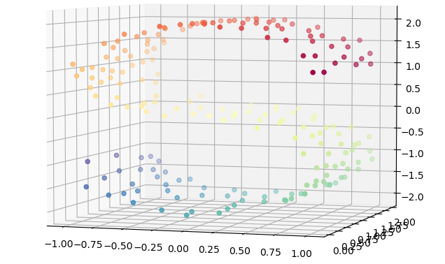
Figure 4. A 10% subset selected with the graph-based estimator. The same void-and-cluster sampling procedure was used.
The notebook also applies the graph estimator to two concentric circles. These are small, visual demonstrations of the idea, not evidence that one neighborhood setting will work for every high-dimensional dataset.
Testing the code
The S-curve example boils down to choosing a density estimator and asking the sampler for ordered indices:
from vc_sample.density_estimation import UMAPDensityEstimator
from vc_sample.void_and_cluster import VoidAndCluster

# X is an array of 2,000 points with three coordinates each.
density = UMAPDensityEstimator(X, n_neighbors=10)
sampler = VoidAndCluster(density, num_points=len(X), num_initial_samples=100)
indices = sampler.sample(size=200)

subset = X[indices]  # 10% of the input points
The result is an ordering of indices into the original data. Taking a prefix gives a smaller subset, which is useful for progressive views. The repository includes setup instructions and the notebooks behind these figures.
What remains difficult
Moving from coordinates to a graph does not make the curse of dimensionality disappear. The quality of the sample depends on whether the graph captures meaningful neighbors. The distance metric, the number of neighbors, and the data’s shape all matter. Building that graph also has a cost, and the current code is a research prototype rather than a benchmarked general-purpose sampler.
What I find useful about the experiment is the division of labor: one component describes local relationships, and the void-and-cluster procedure turns those relationships into a spaced, ordered subset. The S-curve shows why that division matters. A better neighborhood model can make the same sampling procedure useful beyond the spatial and temporal settings that motivated the original work.