Running a language model locally usually means one user and one stream of tokens. Throughput hardly matters in that setting; what you notice is how long each new token takes. This post is about that number, the time per token at batch size one, for Llama 3.2 1B on a small consumer GPU: an 8 GB GeForce RTX 3050. It describes TileInfer, a runtime I built to answer one question: how close can a single persistent kernel get to the time the hardware needs just to read the model?
1. Motivation: one token at a time on a small GPU
At batch size one, a token is a long chain of small, dependent steps. Normalize the hidden state, project it, attend over the earlier tokens, project again, run the MLP; repeat for 16 layers; then compute the logits for the whole vocabulary. Each step streams its weights from DRAM and does very little arithmetic with them (Section 2), and no step can start before the one it depends on has finished.
The usual runtimes run each of these steps as its own kernel. For this model, PyTorch launches 787 kernels per token and llama.cpp 213 (Section 6). Between and inside those kernels the GPU stops streaming. Launches leave gaps. A kernel’s last blocks run while most SMs already sit idle. And the next kernel cannot start loading its weights until the previous one has finished, even though the weights never depend on the token.
The alternative is to run the whole token as one persistent kernel whose work is planned ahead of time: a megakernel. In a previous post I traced persistent threads and megakernels from ray tracing to LLM inference. The closest prior art for this post is Hazy Research’s “Look Ma, No Bubbles!”, a megakernel for the same model at batch size one on H100 and B200 GPUs. It used 78% of the H100’s memory bandwidth and ran more than 1.5 times faster than SGLang, which already uses CUDA Graphs. The name bubbles for the idle time between and inside kernels is theirs. Their kernel runs an instruction interpreter on every SM, pages shared memory so that the next instruction’s weights load while the current one finishes, and tracks dependencies with counters in global memory.
My setup differs from theirs in ways that change the question (Figure 1). The first difference is the floor. A token must read 2.47 GB of weights. At an H100’s 3.35 TB/s that takes about 0.74 ms, and on a B200 about 0.3 ms. Hazy Research measured a kernel launch at about 1.3 µs even inside a CUDA Graph; with a hundred or more kernels per token, microseconds become a large share of a sub-millisecond floor. On the RTX 3050 the same bytes take 11.6 ms (Section 2), and the same microseconds are a few percent of it. The second difference is how hard it is to reach full bandwidth. Terabytes per second need many SMs with deep asynchronous load pipelines. On the RTX 3050, 8 of its 20 SMs already saturate DRAM, and the rest have time to spare (Section 3). The third difference follows from the first two: the scheduling can be simpler. Instead of dynamic counters, TileInfer uses a fixed plan of waves separated by grid barriers (Section 4).
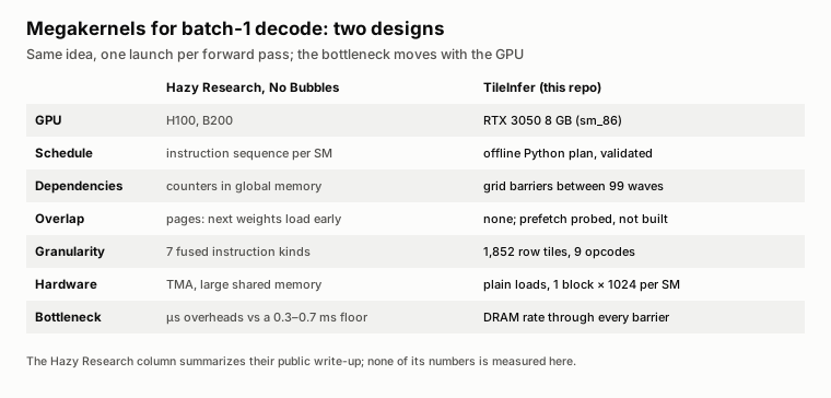
Figure 1. Two megakernels for batch-one decode of the same model. The left column summarizes Hazy Research’s public write-up; none of its numbers is measured here. The right column is the design this post describes.
This is a different regime, not a contest: nothing here is measured against their numbers. The question becomes: on a GPU where the floor is about 16 times longer, does a megakernel still pay, and how close to the floor can one statically scheduled kernel get? TileInfer’s answer has two halves. An offline planner in Python cuts the token into small tile tasks and assigns every task to a fixed worker. One persistent CUDA kernel executes that plan for each token and makes no scheduling decision of its own.
The rest of the post follows the token: where the floor comes from (Section 2), what the RTX 3050 asks of the design (Section 3), how the plan is built (Section 4), what one token looks like on the GPU (Section 5), and how the result compares with PyTorch and llama.cpp (Section 6).
2. Why decode has a lower bound
Token n + 1 needs token n: the model’s output at one position is its input at the next, so there is no parallelism across the sequence. Every token therefore runs the whole model once and reads every weight once. In BF16, Llama 3.2 1B has 2,471,628,800 bytes of weights.
At batch size one, every weight matmul is a matrix-vector product, a GEMV. Each two-byte weight is used for exactly one multiply-add, about one floating-point operation per byte. A GPU needs tens of operations per byte before arithmetic becomes the limit, so decode at batch size one is limited by memory bandwidth, not by compute. Servers raise the operations per byte by batching many users or by verifying several speculative tokens at once; both are out of scope here.
That makes the time to stream the bytes a hard lower bound, the floor. At the RTX 3050’s measured streaming rate of 212.9 GB/s, the weights alone take 11.6 ms per token. Attention adds the key/value (K/V) cache: 32 KiB for each position in the context, 134 MB at 4,096 tokens, which raises the floor to 12.24 ms. Throughout this post, every latency is reported next to its share of the floor.
Figure 2 shows the model as bytes rather than as an architecture diagram. Its 1.24 billion parameters are 79% decoder layers and 21% embedding table. The embedding is tied: the same 128,256 × 2,048 matrix maps the input token to a vector and the final hidden state to logits. The input side reads one 4 KB row. The output side, lm_head, needs one dot product per vocabulary entry and streams the whole 525 MB matrix every token, a fifth of all traffic. The 16 layers form a strict chain. Their order cannot change; only the work inside each step can be spread across SMs.
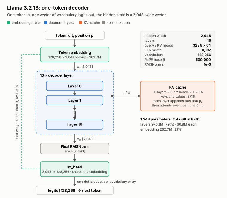
Figure 2. Llama 3.2 1B as a one-token decoder. One token goes in, one vector of 128,256 logits comes out; between them the hidden state is a 2,048-wide vector. The K/V cache is the only state carried from one token to the next.
The K/V cache is the only state carried between tokens. Llama 3.2 uses grouped-query attention: its 32 query heads share 8 K/V heads, which keeps the cache at a quarter of the size it would otherwise have.
Figure 3 walks through one layer. Its seven weight matmuls hold 121.6 MB and take nearly all of the layer’s time; the MLP alone is 83% of the bytes. The other operations, two RMSNorms, the rotary position embedding (RoPE), the SiLU gate and the residual adds, move almost no bytes. But each is a dependency, and each norm is a reduction over the whole hidden vector, so every worker must wait for the complete result of the previous step. Attention is the only cost that grows with the position in the sequence.
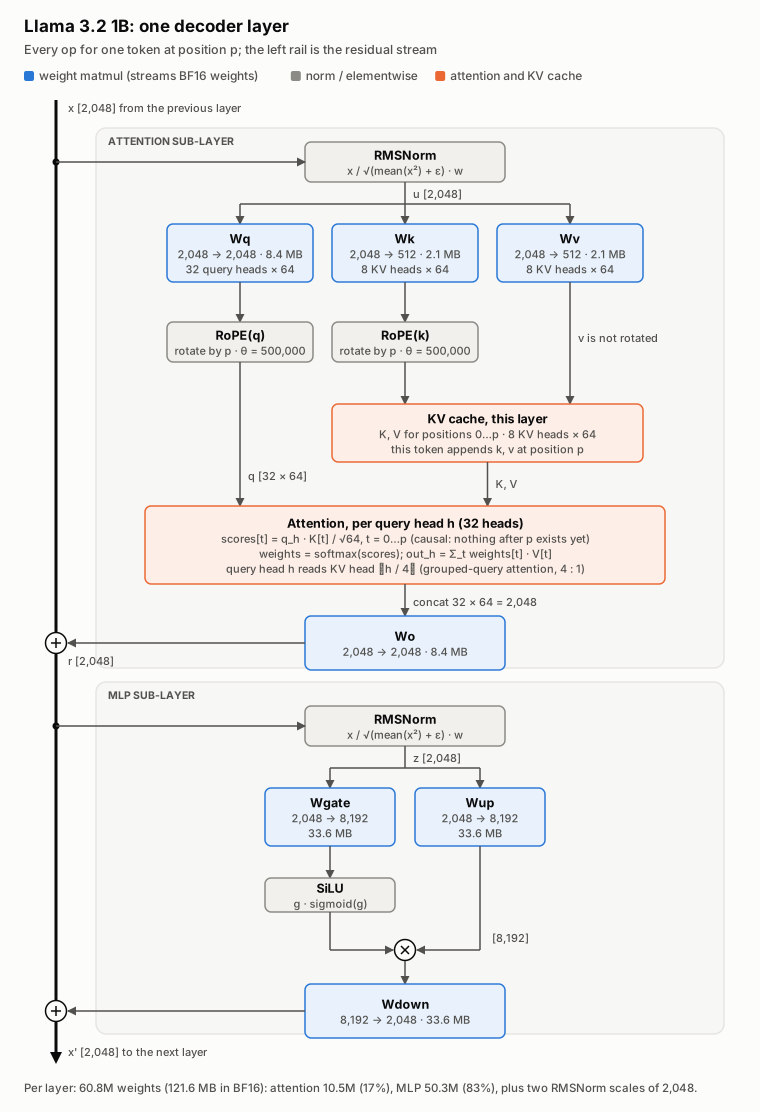
Figure 3. One decoder layer, every operation for one token at position p. Weight matmuls stream BF16 weights; norms and elementwise operations move almost no bytes but each depends on its predecessor.
Every dependency arrow in Figure 3 is a place where the GPU can stop streaming: one piece of work has to finish before the next can start, and DRAM is idle in between. These are the bubbles of Section 1. With seven matmuls and a handful of small operations per layer, a token has well over a hundred of them, and the rest of this post is about not losing time at them.
3. The RTX 3050
The RTX 3050 is an Ampere GPU of compute capability 8.6 with 20 SMs, a 1.5 MB L2 cache and 8 GB of GDDR6 on a 128-bit bus. Its nominal bandwidth is 224 GB/s; a streaming-read benchmark measures 212.9 GB/s, about 95% of it. That measured number is the yardstick for everything that follows. Figure 4 collects what the card means for the design.
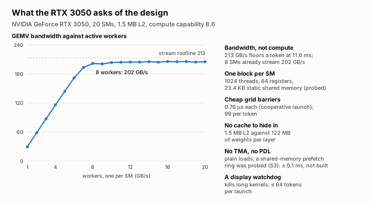
Figure 4. What the RTX 3050 asks of the design. Left: the bandwidth of the decoder’s GEMV against the number of active workers, one per SM; eight workers already stream 202 GB/s.
Bandwidth comes from a few SMs. One SM streams about 30 GB/s, so eight of the 20 SMs come close to saturating DRAM. The other twelve are slack: there is spare compute for norms, attention and epilogues, as long as the weight stream keeps going. The kernel uses one block of 1,024 threads per SM, which the probe of the compiled kernel confirms fits.
Nothing stays in cache. A 1.5 MB L2 against 122 MB of weights per layer means every weight comes from DRAM on every token. There is no reuse to exploit across tokens, only bandwidth to keep busy.
Grid barriers are cheap. A barrier across all 20 blocks of a cooperative launch costs under a microsecond when nobody is late. A token has up to 99 of them, so their pure latency is about 0.1 ms. The real cost of a barrier is that the slowest worker sets the pace for everyone, which is why the plan in Section 4 balances bytes, not tasks.
Plain loads. Ampere has no Tensor Memory Accelerator (TMA) and no programmatic dependent launch. The worker streams weights with ordinary vectorized loads. I tried a shared-memory ring that would keep loading the next task’s weights while a worker waits at a barrier; on this GPU, weights prefetched before a barrier hid none of the time lost around it, and the best case was about 0.1 ms per token.
A tight register budget. The worker runs at 64 registers per thread. Values that change at run time must not reach the hot loops as extra registers or as divisions: while moving the token loop into the kernel (Section 5), passing the sequence position at run time first cost up to 0.45 ms per token, until it no longer forced local-memory copies and 64-bit divisions into code that every task runs.
4. Tile-based static scheduling
Figure 5 shows the split between planning and execution. Python plans once per model and GPU, offline. First it probes the compiled worker kernel for the facts the plan depends on: one block of 1,024 threads per SM, 64 registers per thread, 20 workers. Then it imports the checkpoint and writes a package: the plan, the packed BF16 weights and the target description. The C++/CUDA runtime loads that package, validates it again, and executes it with one cooperative launch. At run time it makes no scheduling decision.
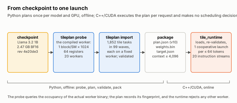
Figure 5. From checkpoint to one launch. The probe queries the occupancy of the actual worker binary; the plan records its fingerprint, and the runtime rejects any other worker.
The plan for Llama 3.2 1B has 1,852 tile tasks in 99 waves. A task is one opcode, one of nine, applied to a range of output rows, with validated operands. Each task belongs to exactly one wave and one worker. The runtime checks before launch that every buffer range is in bounds, that every output row has exactly one writer, that no task runs before the tasks it reads from, and that the plan was made for this worker binary and this GPU.
Figure 6 shows how one layer becomes tiles. The rule is simple: split rows evenly over the 20 workers, and fold the small operations into the tasks next to them.
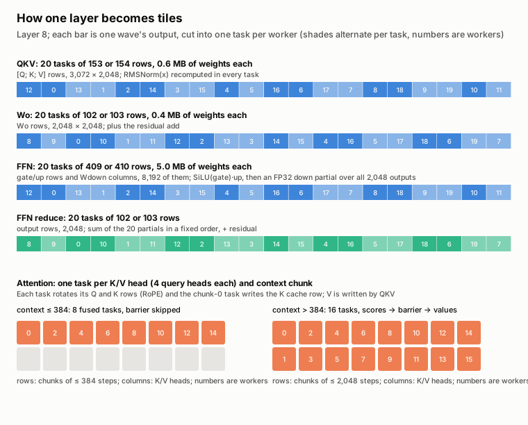
Figure 6. How one layer becomes tiles. Each bar is one wave’s output cut into one task per worker; numbers are workers.
- QKV. The stacked Q, K and V projections are 3,072 rows of 2,048 weights. Each of the 20 tasks takes 153 or 154 rows, 0.6 MB of weights. Each task recomputes the RMSNorm of the 2,048-wide input itself. That repeats a 4 KB read and a reduction 20 times, but it replaces a separate norm wave and its barrier.
- Attention. One task per K/V head, covering its four query heads, and per context chunk. The task applies RoPE to its Q and K rows and writes the new K row to the cache; QKV already wrote the V row. Up to 384 tokens of context, eight tasks each compute scores and values in one pass. Beyond that, 16 tasks split the context into two chunks, and a barrier separates the scores from the values.
- Wo. 20 tasks of 102 or 103 rows merge the attention partials, project them, and add the residual.
- FFN. Each worker owns 409 or 410 of the 8,192 intermediate rows. It computes its rows of the gate and up projections, applies SiLU(gate) · up, and multiplies the result by its matching columns of the down projection. That produces an FP32 partial sum for all 2,048 outputs, 5.0 MB of weights per task, with no barrier between the up and down projections.
- FFN reduce. 20 tasks of 102 or 103 output rows sum the 20 partials in a fixed order and add the residual. A fixed order means no atomics, and the result is the same bits on every run.
Figure 7 shows the resulting waves. A wave depends only on earlier waves and ends at a grid barrier. Each layer has six: QKV, scores, values, Wo, FFN and FFN reduce. Together with the embedding, the final norm and lm_head, a token is 1 + 16 × 6 + 2 = 99 waves. The one barrier that changes with the input is the one between scores and values. Up to 384 tokens of context, the attention work is small enough to finish in one pass, so the kernel skips that barrier.
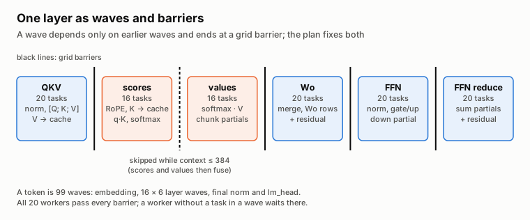
Figure 7. One layer as waves and barriers. All 20 workers pass every barrier; a worker without a task in a wave waits there.
Figure 8 shows the static assignment at a context of 4,096. In each weight wave, every worker streams the same number of bytes, to within 1%, because the planner balances rows by construction. Attention is the visible exception: it has 8 or 16 tasks, so 4 to 12 workers have nothing to do and wait at the barrier. That is cheap here, for the reason Section 3 gave: attention moves few bytes compared with the weight waves, and the idle SMs are the slack the GPU has anyway. Recomputing the norm in every QKV task is affordable for the same reason.
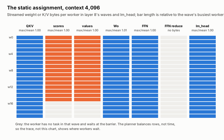
Figure 8. The static assignment at context 4,096: streamed weight or K/V bytes per worker in layer 8’s waves and in lm_head. Grey marks a worker with no task in that wave. The planner balances rows, not time, so the trace in Section 5 shows where workers actually wait.
This is where the design parts from Hazy Research’s. Their kernel decides at run time when an instruction may start, using counters, and overlaps the next instruction’s loads with the current one. TileInfer fixes every task, every byte and every barrier before launch. That buys three things. The plan can be validated completely before it runs. The results are bit-reproducible, since every reduction has a fixed order. And every cost is known in advance, so a timeline can be read against the plan. What it costs is overlap: no work crosses a barrier. On this GPU that cost is small. The prefetch probe of Section 3 bounded the gain from overlapping weight loads with barriers at about 0.1 ms per token, and a later probe of counter waits in place of the barriers around attention also did not pay.
5. One token, end to end
Figure 9 shows a whole token as the GPU executes it, at contexts 1 and 4,096. Each row is a worker; time runs to the right; layer 8 is enlarged below.
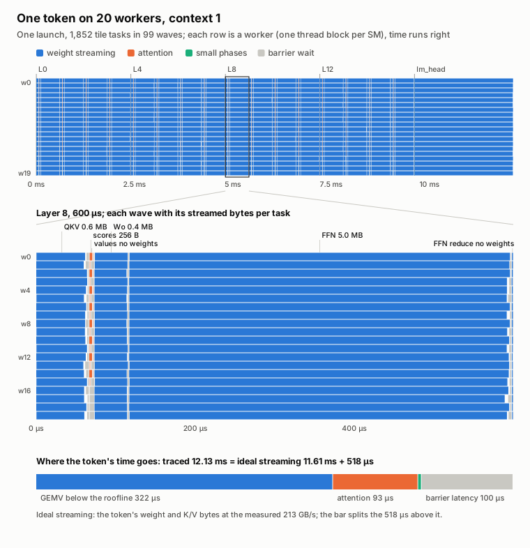
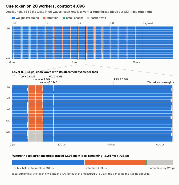
Figure 9. One token on 20 workers at context 1 (top) and 4,096 (bottom). Ideal streaming is the token’s weight and K/V bytes at the measured 212.9 GB/s; the bar at the bottom of each panel splits the time above it.
At context 1 the traced token takes 12.13 ms, 518 µs above ideal streaming. Most of that, 322 µs, is GEMV running below the bandwidth roofline: QKV and Wo stream at 190 GB/s, the FFN and lm_head at 209 GB/s. QKV (85 µs), the FFN (106 µs) and Wo (51 µs) hold most of this excess. Barrier latency adds 100 µs and attention 93 µs. The small operations folded into other tasks cost 4 µs in total.
At context 4,096 the token takes 12.98 ms, 738 µs above ideal streaming. The GEMV loss stays about the same at 331 µs, and barriers add 120 µs. Attention grows to 283 µs. It reads the K/V cache at 141 GB/s, below the rate of the weight waves, with 16 of the 20 workers taking part.
Figure 10 shows the loop around these tokens. One launch decodes up to 64 consecutive tokens, with a grid barrier between them. Greedy selection runs inside the kernel. Each lm_head task writes the best candidate of its rows, the largest logit with the lowest token ID among ties, into its own slot. At the start of the next step, every worker reads all 20 slots and combines them. Because all workers read the same slots, they all arrive at the same token and the same decision to stop, without a counter or an extra barrier. Worker 0 records the token, the count and the end-of-sequence flag; a non-finite logit sets an error word and stops the request. The host only launches the kernel and reads the results; it does not take part in choosing the next token.
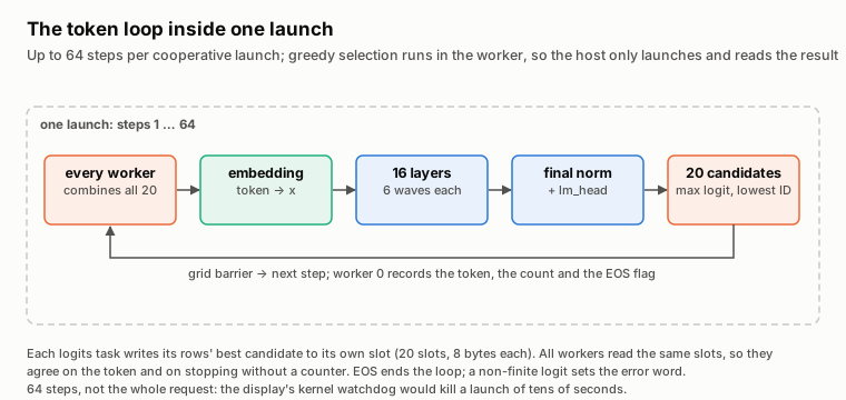
Figure 10. The token loop inside one launch. Up to 64 steps run per cooperative launch; greedy selection runs in the worker.
6. Against PyTorch and llama.cpp
All runtimes run the same Llama 3.2 1B base checkpoint with BF16 weights at batch size one. A fixed-context measurement stops when the logits are ready, with no sampling. PyTorch runs Hugging Face Transformers with eager attention, once launching kernels as it goes (eager) and once replaying a CUDA Graph. llama.cpp runs a GGUF conversion of the same weights with flash attention and float16 or BF16 K/V. Every runtime stays resident in its own process while measurement blocks interleave, with medians over both spawn orders, at locked GPU clocks. llama.cpp is timed on the host around its synchronous decode call, the others with CUDA events.
Figure 11 shows the result. TileInfer takes 12.13 ms per token at context 1 and 12.99 ms at 4,096: 96% and 94% of the floor (11.61 and 12.24 ms). CUDA Graph replay takes 12.84 and 20.34 ms, so TileInfer needs 5.6% and 36% less time. llama.cpp with float16 K/V takes 13.68 and 14.32 ms; TileInfer needs 11% and 9% less time. PyTorch eager takes 13.96 and 21.48 ms. Every paired difference against TileInfer has a 95% confidence half-width of 3 to 12 µs.
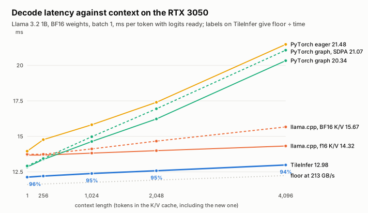
Figure 11. Decode latency against context on the RTX 3050: ms per token with the logits ready. Labels on TileInfer give floor ÷ time.
Generating 64 tokens from a short prompt, with greedy selection included, gives the same order: TileInfer 82.3 tokens per second, graph replay 76.4, llama.cpp 71.8 and PyTorch eager 69.3. All runtimes produce the same 64 tokens.
Figure 12 shows why the baselines are slower. It traces one token of each runtime in Nsight Systems, from the previous token’s last kernel through the next token.
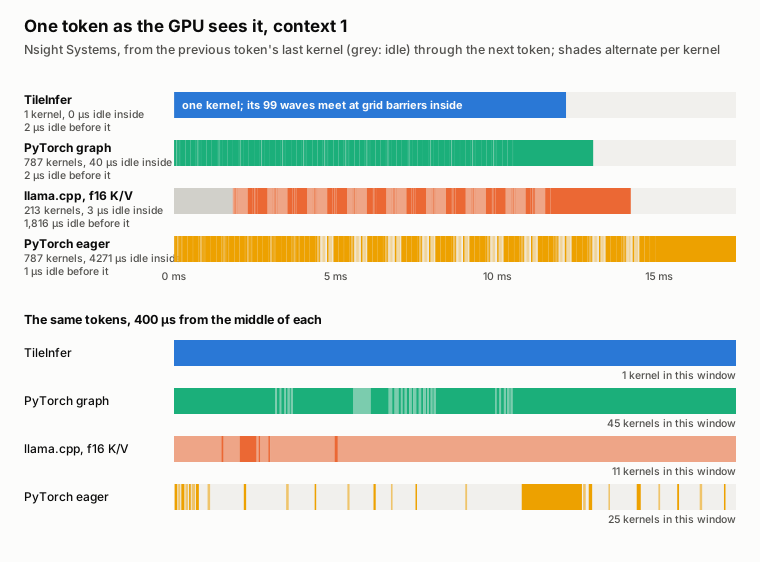
Figure 12. One token as the GPU sees it, at context 1. Grey is idle time; shades alternate per kernel. Below, 400 µs from the middle of each token.
PyTorch eager runs 787 kernels per token, and the host launches each one, so the GPU waits between them.
PyTorch graph replay runs the same 787 kernels with only 40 µs of idle time between them. CUDA Graphs remove the launch gaps, as they should. What is left is inside the kernels: blocks ramping up and draining at the start and end of each kernel, GEMV shapes that the library kernels run below the roofline, and eager attention, which expands the eight K/V heads to 32 before its matmuls. That last cost grows with the context, which is why graph replay falls from 90% of the floor at context 1 to 60% at 4,096.
llama.cpp runs 213 kernels per token with only a few microseconds idle between them, then 1.8 ms idle before the next token starts. In that gap, one 513 KB device-to-host copy of the float32 logits takes 1.19 ms. Its flash attention scales well with context, so this loss is nearly constant per token, and llama.cpp overtakes graph replay between 256 and 1,024 tokens of context. To be fair to it: in the fixed-context measurement, TileInfer and PyTorch leave the logits on the GPU, while llama.cpp’s API returns them on the host. The generation numbers are the like-for-like comparison, and there llama.cpp takes 15% longer per token than TileInfer. Why the copy runs at only 0.43 GB/s I have not examined; a pageable host buffer is the likely cause.
TileInfer runs one kernel with nothing idle between tokens. Its losses are inside that kernel, and Section 5 accounts for them.
These are end-to-end comparisons of whole runtimes. PyTorch and llama.cpp use different kernels and different fusions as well as a different execution model, so the numbers do not isolate static scheduling as the cause of the difference. What they do show is where each runtime’s time goes, and that one launch per 64 tokens leaves no gaps for the host or the launch machinery to fill.
The results also agree. At every measured context, every runtime picks the same next token. TileInfer matches Hugging Face eager attention in BF16 within calibrated tolerances. Over a 27-step check, greedy selection agrees at 26 steps; the remaining step is a near-tie in the reference, whose top two logits differ by only 0.125. llama.cpp’s teacher-forced comparison against Transformers shows no real mismatches.
That answers the question from Section 1. On the RTX 3050 the floor is about 16 times longer than on an H100, so the bubbles are only a few percent of a token. A single statically planned kernel removes most of them: TileInfer runs at 94 to 96% of the bandwidth floor at every measured context, and what remains is mostly GEMV running slightly below the roofline.
Appendix
The code is in the Tiles repository. One command, experiments/showcase/showcase.py run, builds the runtime, probes the GPU, imports the pinned checkpoint, runs the checks and every measurement in this post against llama.cpp tag b11871 and PyTorch, and redraws the figures.
Two more figures answer common questions. Figure A1 is the 4,096-token version of Figure 12; Figure A2 is the context-1 version of Figure 8.
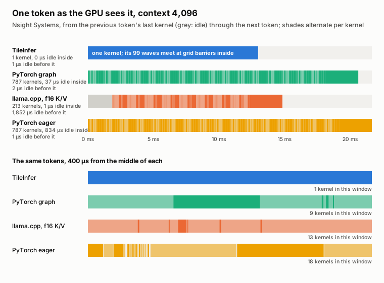
Figure A1. One token as the GPU sees it, at context 4,096.
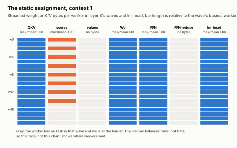
Figure A2. The static assignment at context 1. Attention runs as eight fused tasks, so twelve workers wait at its barrier.