Reading about recent megakernels for LLM inference brought me back to persistent threads and megakernels I used in my own GPU work. This post traces both ideas from their origins in ray tracing to modern attention kernels and full-model LLM inference

Work scheduling determines how a parallel workload is distributed among processors and when dependent tasks can execute. GPUs are easiest to keep busy when work can be divided into many independent tasks of similar size. When tasks differ in duration or generate new work, a fixed assignment can leave some processors idle while others remain busy. Persistent threads and megakernels give GPU programs more control over work assignment and execution across stages. This control offers opportunities to improve load balance and data locality, but also introduces coordination overhead and additional resource demands.

These techniques also apply to low-latency inference, where kernel launch overhead and gaps between short, dependent operations contribute to execution time. Seeing these ideas take on a new role is exciting, and I want to trace how they developed, what problems they solve, and when the extra control is worth its cost.

1. Dynamic Scheduling on the GPU

Ray tracing provides a concrete example of uneven work: some rays need only a few intersection tests, while others require a long search through the scene. Assigning one ray to each GPU thread therefore produces different execution times. Threads execute in groups called warps, following the single-instruction, multiple-thread (SIMT) model. When threads take different branches, each path executes with only the participating threads active. This is warp divergence; threads that finish their rays early also become inactive while others continue.

At a coarser level, hardware assigns thread blocks to streaming multiprocessors (SMs) as resources become available. This distributes blocks across the GPU, but does not reassign rays within a running block. Aila and Laine (2009) found that uneven ray workloads also exposed inefficiencies in the GTX 285’s hardware work distributor. Their solution was to launch enough workers to fill the GPU, then let those workers repeatedly fetch batches of rays from a shared pool. Keeping workers alive across successive assignments gave software control over work distribution, although divergence within each batch remained. Gupta, Stuart, and Owens (2012) later studied this persistent-thread approach across a broader range of workloads, examining its benefits and scheduling costs.

Numerically integrating differential equations produces a similar problem. Each thread might follow a particle through a flow field, with adaptive step sizes and different stopping conditions giving each trajectory a different amount of work. The trajectories also access different parts of the field, producing scattered memory accesses. Managing this imbalance and data access was a major challenge in my work on visualizing stochastic differential equations. If the field is partitioned across GPUs or nodes, access to remote data adds communication costs. Work assignment must then consider both the amount of computation and the location of its input data.

2. Persistent threads and megakernels

In the ray-tracing example, a fixed number of workers stays active and processes successive batches of rays within one kernel launch. This reuse is what makes the execution persistent. A worker can be a thread, a warp, or an entire block, depending on how many threads cooperate on each task. Software decides which work comes next, while the hardware continues to schedule and execute the workers’ instructions.

In contrast to the ray-tracing example, a rasterization pipeline contains different kinds of work: preparing triangles, generating samples, and computing their colors. Combining several such stages in one kernel produces a megakernel. Persistence therefore describes how workers are reused, while the term megakernel describes how much of the pipeline a kernel contains. The combined stages can follow a fixed sequence or be selected during execution as work becomes available.

These choices are independent. Persistent workers can repeatedly perform just one operation, as in FlashInfer’s persistent attention kernels, while a megakernel can combine stages without a persistent worker loop. In inference, neither choice by itself means that model weights remain in fast on-chip memory or that one launch generates multiple tokens.

Whippletree (Steinberger et al., 2014) combines persistence with a megakernel to execute pipelines whose workload changes as they run. Each stage defines a task type, and a queue holds the inputs waiting to be processed by that task. Workers take inputs from these queues and execute the corresponding stages. A stage can also add new inputs to another stage’s queue or to its own, allowing the pipeline to generate further work without another kernel launch.

I used this approach in my CUDA software rasterizer, which converts triangles into pixels while accounting for surface displacement. Its adaptive sampling operation decides where additional samples are needed and adds them to the same stage’s input queue. Those samples begin with the Displace Shader, which evaluates their displaced positions, before returning to adaptive sampling. The orange feedback edge below shows this recursive work generation: workers process the newly queued samples through the same stage again.

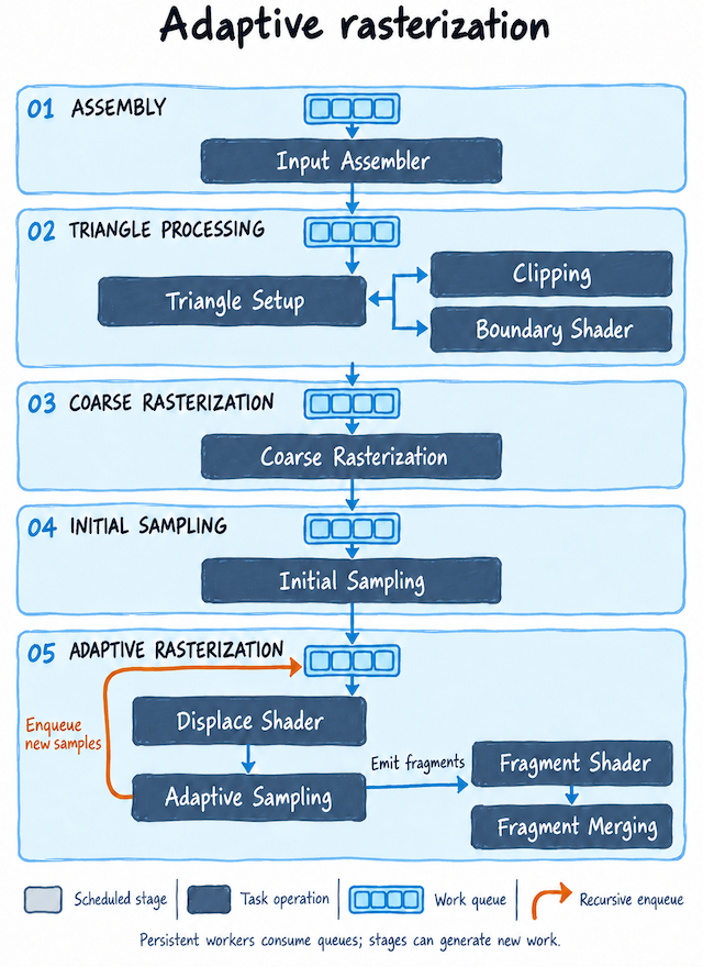
Figure 1. Adaptive rasterization using the Whippletree megakernel framework. Light containers are scheduled stages; dark cards are operations within them. Blue queues hold stage inputs, and the orange edge adds new samples to the adaptive stage’s queue.

3. Why execution boundaries become a latency problem

Uneven work is one reason to take control of GPU scheduling. Another appears when operations are short and dependent: the next operation needs a result from the previous one before it can start. Figures 2 and 3 are Nsight Systems timelines of a tiny transformer generating one token for one sequence (batch size one). Each blue block marks GPU kernel activity. In the PyTorch eager execution shown in Figure 2, the blocks are separated by visible idle intervals. Those intervals add to the critical path, the chain of dependent work that determines when the token is ready. The marked decoding step takes 3.202 ms in this capture.

Figure 2. One token, batch size one, in PyTorch eager mode. The gaps between GPU kernel activities contribute to the 3.20 ms decoding step.

Several costs can create such gaps. The CPU must submit each kernel, which can leave the GPU waiting if submissions arrive too slowly. On the GPU, each launch has setup and scheduling work; in a dependent sequence on one CUDA stream, the next kernel also waits for the previous kernel’s last thread blocks to finish (the tail effect). Across a kernel boundary, intermediate values cannot remain in the previous kernel’s registers or shared memory. They usually pass through global memory, though a cache may serve the next read, and the next kernel must start its own input or weight loads. The timeline shows the gaps, but by itself does not identify how much each cause contributes.

CUDA Graphs reduce launch costs by recording a sequence of GPU operations and replaying it with one CPU submission. Figure 3 shows the same transformer step under graph replay. Its marked duration is 590.333 µs, roughly one-fifth of the eager step in Figure 2. Kernel activity is much more tightly packed, although some gaps remain.

Figure 3. The same single-token, batch-one step replayed as a CUDA Graph takes 590 µs in this capture. Separate kernels and some idle intervals remain visible.

Graph replay helps in real inference systems too: in NVIDIA’s llama.cpp profile, GPU-side launch gaps, rather than CPU submission, limited the measured case, and graphs reduced them. A graph still runs separate kernels, so dependent stages retain their boundaries and cannot pass registers or shared memory directly from one to the next. NVIDIA’s nv-WaveNet implementation took a further step for sequential audio generation: single-kernel designs generate multiple dependent samples per launch, and its persistent variant keeps weights in registers across samples. That removes more boundaries, but makes communication between worker blocks part of the remaining latency. The question is whether the work saved at boundaries exceeds the coordination costs introduced inside the kernel.

4. The price of taking over scheduling

A megakernel removes launch boundaries by putting more stages into one program, but those stages must share its resource budget. In Megakernels Considered Harmful (2013), Laine, Karras, and Aila found that a path tracer with separate, specialized kernels handled complex materials better than a single large kernel. Their result highlights two clear disadvantages: the large kernel uses more registers, and threads following different paths waste execution capacity.

Registers hold a thread’s working values. The register count is set for the whole kernel, so a demanding stage can raise the allocation even while a thread runs a simpler stage. Each streaming multiprocessor (SM) has a finite register file and shared memory capacity. Higher use per thread or block can leave room for fewer resident warps; this fraction of the hardware’s possible active warps is called occupancy. With fewer warps ready to run, the SM has less work to switch to while a memory request is outstanding. Excess register demand can also spill values into slower local memory. Separate kernels let a lean stage use fewer registers and let each stage choose a suitable block size and shared memory allocation. A very large combined program can put pressure on the instruction cache as well.

Combining stages can also increase warp divergence: if lanes of one warp take different stage paths, only the lanes on the current path do useful work. Sorting similar tasks into queues can improve coherence, but fetching and dispatching tasks, updating shared work counters with atomic operations, and synchronizing workers all take time. Coordination across blocks needs particular care. If all resident blocks wait for results from blocks that have not yet been scheduled, the kernel can deadlock. An ordinary launch gives no guarantee that a waiting block’s producer has started, as the CUDA execution model explains. Cooperative launches support grid-wide synchronization within their launch-size and resource limits.

Volta’s Independent Thread Scheduling made some coordination patterns easier. It keeps execution state, including a program counter, per thread, so one lane can wait while another lane in the same warp produces data. Earlier warp-level lock or producer–consumer schemes could deadlock because divergent lanes could not make that kind of independent progress. The hardware still issues instructions to groups of active lanes, so divergent paths remain costly, and per-kernel register and shared memory limits still constrain occupancy. Code must also use explicit synchronization and appropriate atomics rather than assume lanes move in lockstep, as the Volta tuning guide explains. Volta expanded the ways to coordinate workers; whether a megakernel provides a benefit still depends on measuring saved boundaries against its resource and scheduling costs on the target GPU.

5. Modern kernels schedule asynchronous work

Volta’s Independent Thread Scheduling expanded the coordination patterns possible inside a kernel. A matrix multiplication processes inputs in tiles, small chunks that fit in fast on-chip storage. If the kernel waits for each tile before computing, memory latency enters every iteration. CUTLASS uses software pipelining: while computation uses one tile, a second buffer receives the next. Workers track when each buffer is full, consumed, and safe to reuse. This hides latency at the cost of more shared memory, which can reduce occupancy.

The same warps can load and compute, or a kernel can assign those roles to separate warps, a technique called warp specialization. Producer warps initiate transfers; consumer warps perform matrix multiplication and release buffers for reuse. Ampere introduced asynchronous copies, and Hopper’s Tensor Memory Accelerator (TMA) moves tiles between global and shared memory with little instruction or register overhead. Hopper also added asynchronous Tensor Core operations through warpgroup matrix multiply-accumulate (WGMMA). Software assigns the roles and dependencies; hardware schedules ready warps and carries out transfers and arithmetic.

FlashAttention-3 shows how far this can go inside one attention kernel: it overlaps transfers, Tensor Core matrix multiplication, and softmax work on other execution units. Figure 4 sketches the idea. At the middle interval, TMA loads a future tile while Tensor Cores multiply the current tile and CUDA cores work on softmax for an earlier tile. Each tile still follows its dependencies in order; the overlap comes from processing different tiles at once.

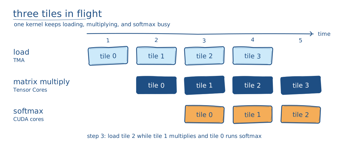
Figure 4. A simplified software pipeline inside one attention kernel, inspired by FlashAttention-3. Tile numbers follow data through loading, matrix multiplication, and softmax; the intervals illustrate overlap, not exact instruction timing.

Keeping several tiles in flight needs buffers and readiness signals. Their live intermediate values also raise register pressure, bringing back the occupancy tradeoff from Section 4. FlashAttention-4 redesigns the pipeline for Blackwell, where faster Tensor Cores shift more attention to softmax and memory traffic.

CUTLASS also has persistent matrix-multiplication kernels whose worker blocks process several output tiles. A megakernel spanning multiple operators extends this scheduling idea: it must decide when different operators may run, communicate their results, and manage their different resource needs. Efficient overlap inside one operator provides a foundation, but the larger schedule still has to earn its coordination cost.

6. From persistent attention to full LLM inference megakernels

During LLM decoding, attention reads the key/value (KV) cache, the stored representations of earlier tokens. Requests in one batch can have very different context lengths, so assigning one fixed amount of work to each GPU block leaves some blocks idle while others process long histories. FlashInfer splits longer histories into chunks and plans how to distribute them among persistent blocks. This is the same load-balancing problem that motivated persistent ray-tracing workers in Section 1, now applied to attention. Its persistent kernel can also combine partial attention with final aggregation, but the scheduling scope remains the attention operator. The plan changes with the requests, while the kernel’s launch size and workspace addresses stay fixed so the computation can participate in CUDA Graph replay. Persistence and graphs can therefore work together.

ThunderMLA makes the scheduling of dependent attention tasks more explicit. For long contexts, blocks compute partial attention results, which must then be reduced into the final output. An instruction list tells the resident workers which partial or reduction task to perform, and a signal in global memory records when a task’s inputs are ready. Both stages run in one kernel. The scheduler can assign work across streaming SMs and overlap a reduction with still-running attention tasks that it does not depend on. It must also pay for the instruction dispatch and synchronization that the separate-kernel version got from its execution boundaries.

At model scope, Hazy Research’s Llama-3.2-1B megakernel (don’t skip this link, it’s a fantastic read!) executes the full forward pass for one token, from the first layer through the output logits, within one launch for batch-one decoding. Each SM follows a prepared sequence of instructions for operations such as projection, attention, and the multilayer perceptron. Dependency counters let a downstream task start when its particular input chunk is ready, without waiting for every block of the preceding operation. The kernel also reuses shared-memory space across instructions and begins loading weights for upcoming work while earlier work finishes.

Those weights still come from GPU global memory. The gain is a steadier stream of loads: fewer pauses for launch boundaries and straggling blocks, and more chances to start the next transfer early. CUDA Graphs reduce CPU submission overhead, but they still replay separate kernels with their dependencies and startup costs. In the authors’ batch-one H100 measurements, the megakernel was more than 1.5 times faster than their SGLang baseline, which already used CUDA Graphs. Of course, this result is specific to the measured model, GPU, and workload; it does not mean a megakernel is always faster.

Writing such schedules by hand becomes difficult as the program grows. Mirage Persistent Kernel (MPK) explores a compiler and runtime approach: it turns tensor programs into a graph of tasks at SM granularity, then executes them with decentralized scheduling inside a persistent megakernel. The task graph makes dependencies and opportunities to overlap operators explicit. Scheduling is still the central problem, but more of it moves from handwritten kernel logic into the compiler and in-kernel runtime.

7. When megakernels might help

Persistence is worth investigating when a profile shows uneven work, short dependent kernels, or idle gaps where memory transfers and computation could overlap. The Nsight timelines in Figures 2 and 3 show why launch gaps matter, but also why CUDA Graphs are an essential baseline: they already remove much of the eager-mode delay. A larger kernel may shorten the remaining gaps, while its register use, lower occupancy, synchronization, and scheduling work can add time elsewhere. The balance changes with model size, batch size, context length, and GPU architecture.

The practical test is to compare an optimized sequence of separate kernels under CUDA Graph replay with the persistent or fused design on the intended workload. Measure latency per generated token alongside occupancy, memory activity, and scheduling overhead. The useful result is a shorter critical path to the token, not simply fewer kernel launches.